Marine ecosystems, from coastal to deep sea, now show the influence of human actions, with coastal marine ecosystems showing both large historical losses of extent and condition as well as rapid ongoing declines (established but incomplete) {2.2.5.2.1, 2.2.7.15}
- Direct exploitation of fish and seafood has the largest relative impact in the oceans (well established) {2.2.6.2}.
- The direct driver with the second highest impact on the oceans is the many changes in the uses of the sea and coast land (well established) {2.2.6.2} (See Summary of Observed Changes)
Distribution Of Changes In The Global Ocean
Source: Halpern (B. S., Walbridge, S., Selkoe, K. A., Kappel, C. V., Micheli, F., D’Agrosa, C., … Watson, R. (2008). A Global Map of Human Impact on Marine Ecosystems. Science, 319(5865), 948–952.doi:10.1126/science.1149345
1. Every square kilometer of the ocean is affected by some anthropogenic driver of ecological change
2. Over 41% of the world’s oceans have medium to very high cumulative impacts:
- North and Norwegian seas, South and East China seas, Eastern Caribbean, North American eastern seaboard, Mediterranean, Persian Gulf, Bering Sea, and the waters around Sri Lanka.
3. Lowest impact areas include high-latitude Arctic and Antarctic poles, but this may change due to future polar ice loss
4. Ecosystems with highest impacts include hard and soft continental shelves and rocky reefs, and coral reefs.
Summary of Observed Changes
Temperature Changes
- Rising sea surface temperatures; reduction in oxygen content; stratification; coral bleaching
- Heat content increasing deeper into the ocean
- Global ocean animal biomass consistently declines with climate change, and that these impacts are amplified at higher trophic levels (Source: Lotze, et al., Global ensemble projections reveal trophic amplification of ocean biomass declines with climate change. http://www.pnas.org/cgi/doi/10.1073/pnas.1900194116) Ocean biomass declines with climate change

Rising Sea Levels (“Looking past the horizon of 2100” Nature Climate Change)
- Thermal expansion (warmer water expands)
- Increased runoff from land-based ice sheets
- Greenland
- Antarctica
- Mountain Glaciers
Changes in the Salinity of Seawater
- Changes to the thermohaline circulation
- Increased likelihood of seawater stratification
Threats to Coastal Populations and Infrastructure
- Salt-water intrusion
- Drowning forests
- Inland migration of wetlands
Arctic Sea Ice is Shrinking
- Warming air temperatures increase rate of melting
- Positive feedback albedo loop
Increasing Ocean Acidity
- Absorption of CO2 from atmosphere
- Impacts to shell-forming species, including coralsAbsorption of CO2 from atmosphere
Land-Based Impacts
1. Inorganic and organic pollutants
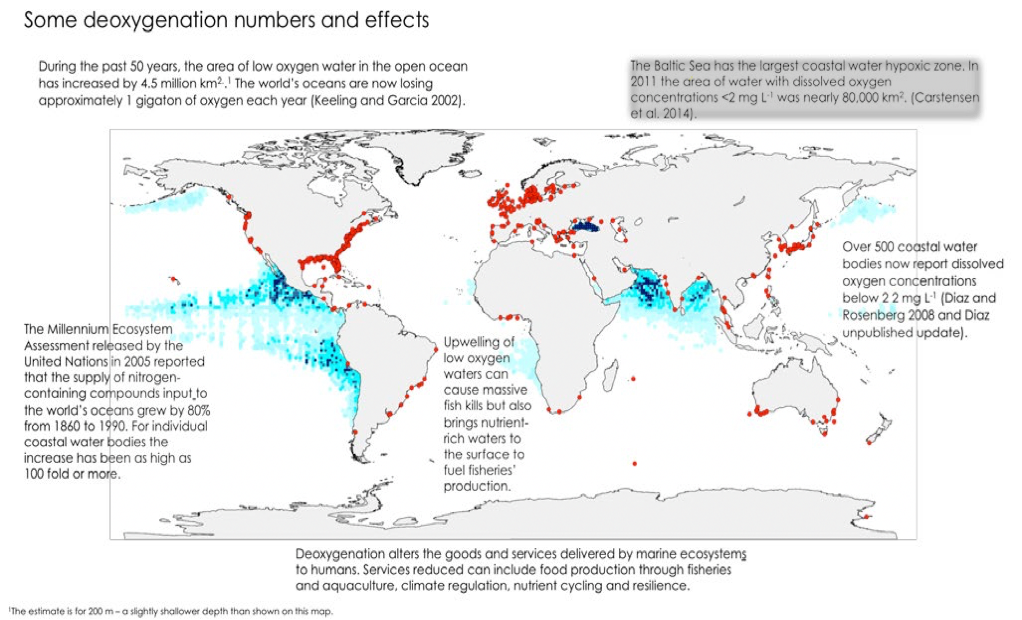
2. Nutrient runoff (point and non-point) and associated hypoxia
3. Aquaculture
4. Invasive species
5. Habitat destruction and alteration; e.g., coastal engineering; tourist development; salt marshes, mangroves, seagrass beds, coral reefs
6. Input and transfer of waterborne pathogens (runoff, aquaculture)
7. Air pollution
a. Toxic chemicals; e.g., POP’s over the Arctic zone by airborne volatilization;
b. Mercury
Source: Lavoie, R.A., Bouffard, A., Maranger, R., Amyot, M., 2018. Mercury transport and human exposure from global marine fisheries. Sci. Rep. 8, 6705.
Significance: Human activities have increased the global circulation of mercury, a potent neurotoxin. Mercury can be converted into methylmercury, which biomagnifies along aquatic food chains and leads to high exposure in fish-eating populations.
Trends: Mercury export from the ocean increased over time as a function of fishing pressure, especially on upper-trophic-level organisms. In 2014, over 13 metric tonnes of mercury were exported from the ocean. Asian countries were important contributors of mercury export in the last decades and the western Pacific Ocean was identified as the main source.
Estimates of per capita mercury exposure through fish consumption showed that populations in 38% of the 175 countries assessed, mainly insular and developing nations, were exposed to doses of methylmercury above governmental thresholds.
Given the high mercury intake through seafood consumption observed in several understudied yet vulnerable coastal communities, we recommend a comprehensive assessment of the health exposure risk of those populations.
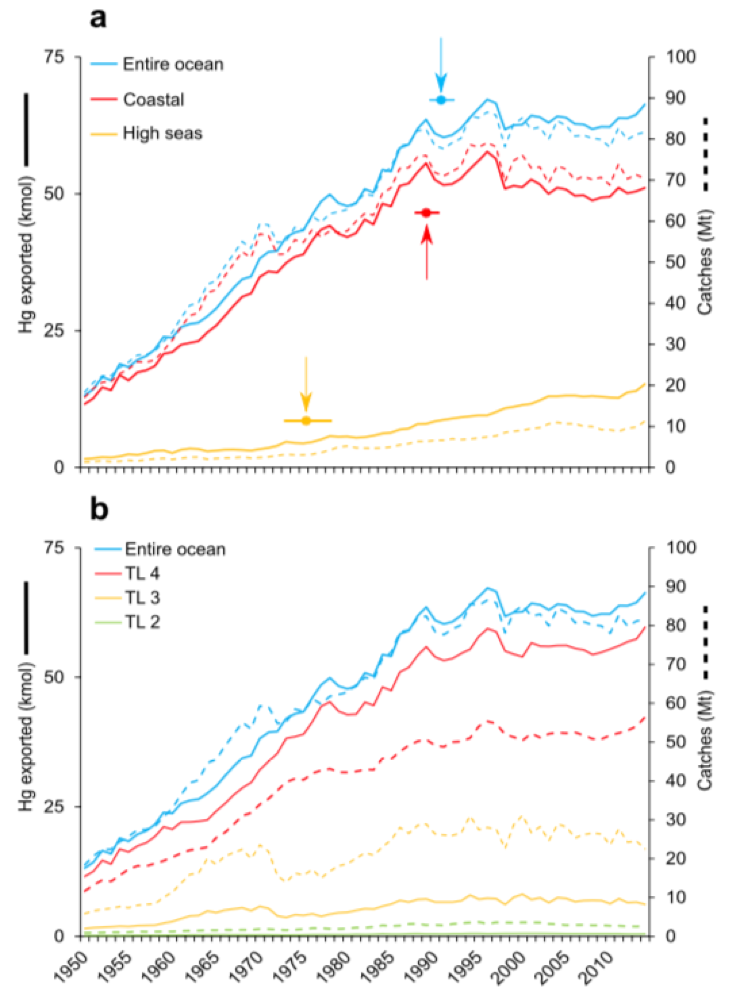
Temporal trends (1950‒2014) of marine fisheries catches (dashed lines) and mercury exported (full lines). (a) Entire ocean (blue) and coastal (red) and high seas (orange) with breakpoint (circle) ± standard error (horizontal line). (b) Entire ocean (blue) and trophic levels (TL) rounded to the nearest integer: 4 (red), 3 (orange), and 2 (green).
Nutrients (N,P): Eutrophication, Dead Zones
Plastics (shipping, fishing, land-based sources)
- Microplastics (nanoparticles; food chain)
- Macroplastics (ingestion, entanglement, habitat loss (shorelines))
- Great Pacific Garbage Patch
Source: Lebreton, L, Slat, B, Ferrari, F, Sainte-Rose, B, Aitken, J, Marthouse, R, Hajbane, S, Cunsolo, S, Schwarz, A, Levivier, A, Noble, K, Debeljak, P, Maral, H, Schoeneich-Argent, R, Brambini, R & Reisser, J 2018, ‘Evidence that the Great Pacific Garbage Patch is rapidly accumulating plastic‘, Scientific Reports, vol. 8, no. 4666. https://doi.org/10.1038/s41598-018-22939-w
- Ocean plastic can persist in sea surface waters, eventually accumulating in remote areas of the world’s oceans.
- Our model, calibrated with data from multi-vessel and aircraft surveys, predicted at least 79 (45–129) thousand tonnes of ocean plastic are floating inside an area of 1.6 million km2; a figure four to sixteen times higher than previously reported.
- Over three-quarters of the GPGP mass was carried by debris larger than 5 cm and at least 46% was comprised of fishing nets. Microplastics accounted for 8% of the total mass but 94% of the estimated 1.8 (1.1–3.6) trillion pieces floating in the area.
- Plastic collected during our study has specific characteristics such as small surface-to-volume ratio, indicating that only certain types of debris have the capacity to persist and accumulate at the surface of the GPGP.
Finally, our results suggest that ocean plastic pollution within the GPGP is increasing exponentially and at a faster rate than the surrounding waters.

Decadal evolution of microplastic concentration in the GPGP. Mean (circles) and standard error (whiskers) of microplastic mass concentrations measured by surface net tows conducted in different decades, within (light blue) and around (dark grey) the GPGP. Dashed lines are exponential fits to the averages expressed in g km−2: f(x) = exp(a*x) + b, with x expressed in number of years after 1900, a = 0.06121, b = 151.3, R2 = 0.92 for within GPGP and a = 0.04903, b = −7.138, R2 = 0.78 for around the GPGP.
Land Loss in Coastal Areas
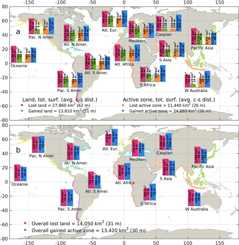
Source: Mentaschi, et al., Global long-term observations of coastal erosion and accretion, Scientific Reports volume 8, Article number: 12876 (2018) https://www.nature.com/articles/s41598-018-30904-w
On a global scale, between 1984 and 2015, the loss of permanent land in coastal areas amounts to almost 28,000 km2, roughly equivalent to the surface area of Haiti (Fig. a). This is almost twice as large as the surface of gained land (about 14,000 km2) over the same period. On the other hand, the overall surface of gained active zone (about 25,000 km2) is more than two times larger than the surface of lost active zone (about 11,500 km2). Overall, the gain of active zone roughly balances the loss of land, and the gain of land balances the loss of active zone. This translates into a net loss of approximately 14,000 km2 of surface for human settlements and terrestrial ecosystems (Fig. b).
Source: Mentaschi, et al., Global long-term observations of coastal erosion and accretion, Scientific Reports volume 8, Article number: 12876 (2018)
On a global scale, between 1984 and 2015, the loss of permanent land in coastal areas amounts to almost 28,000 km2, roughly equivalent to the surface area of Haiti (Fig. a). This is almost twice as large as the surface of gained land (about 14,000 km2) over the same period. On the other hand, the overall surface of gained active zone (about 25,000 km2) is more than two times larger than the surface of lost active zone (about 11,500 km2). Overall, the gain of active zone roughly balances the loss of land, and the gain of land balances the loss of active zone. This translates into a net loss of approximately 14,000 km2 of surface for human settlements and terrestrial ecosystems (Fig. b).
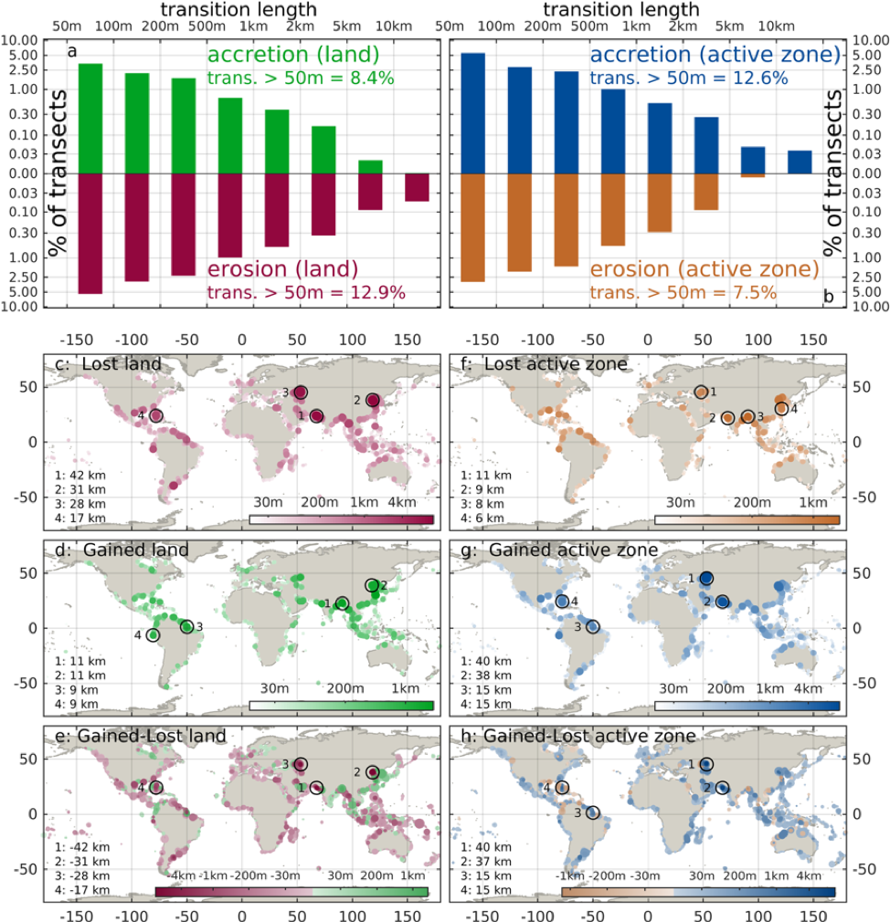
Size distribution of cross-shore transition length above 50 m, for erosion and accretion of land (a) and active zone (b). Lost (c) and gained (d) land around the world; lost (f) and gained (g) active zone; balance gained – lost land (e) and active zone (h). Maps show the length of cross-shore erosion and accretion aggregated on coastal segments of 100 km. In all the maps the 4 spots with the highest local transition along a 250 m transect are indicated.
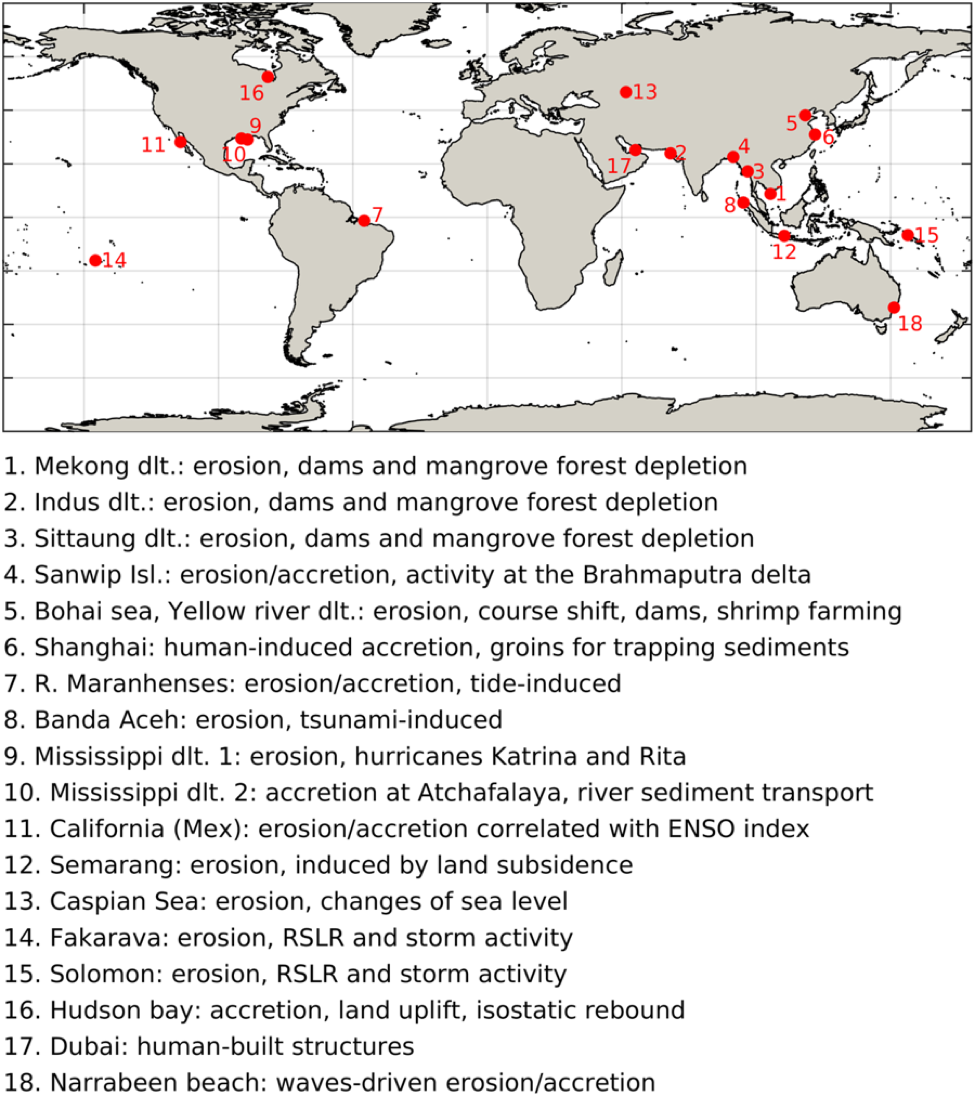
Drivers of shoreline change around the world
Land Loss in Coastal Areas: Shoreline modification “masks” true rates of shoreline change along the Atlantic Seaboard
Source: Armstrong, S. B., & Lazarus, E. D. ( 2019). Masked shoreline erosion at large spatial scales as a collective effect of beach nourishment. Earth’s Future, 7, 74– 84. https://doi.org/10.1029/2018EF001070
(R)ecent rates of shoreline change along the U.S. Atlantic Coast are, on average, less erosional than historical rates. This shift has occurred despite evidence of intensified environmental forcing, including acceleration in rates of relative sea‐level rise and increased significant wave height in offshore wave climates. We suggest that the use, since the 1960s, of beach nourishment as the predominant form of mitigation against chronic coastal erosion in the United States…could explain the unexpected reversal in shoreline‐change trends.
Using U.S. Geological Survey shoreline records from 1830–2007 spanning more than 2,500 km of the U.S. Atlantic Coast, we calculate a mean rate of shoreline change, prior to 1960, of −55 cm/year (a negative rate denotes erosion). After 1960, the mean rate reverses to approximately +5 cm/year, indicating widespread apparent accretion despite steady (and, in some places, accelerated) sea‐level rise over the same period.
Cumulative sediment input from decades of beach‐nourishment projects may have sufficiently altered shoreline position to mask “true” rates of shoreline change. Our analysis suggests that long‐term rates of shoreline change typically used to assess coastal hazard may be systematically underestimated. We also suggest that the overall effect of beach nourishment along of the U.S. Atlantic Coast is extensive enough to constitute a quantitative signature of coastal geoengineering and may serve as a bellwether for nourishment‐dominated shorelines elsewhere in the world.